Differentiable 3D Mesh Fitting: From Sphere to Accurate Mesh in 60 Minutes
Stack: PyTorch, PyTorch3D, Python · GitHub link · For a condensed version of this post see the README.
Table of Contents
- The Problem
- Workflow Overview
- Key Design Decisions & Techniques
- Results & Reflections
- 3D Vision vs. Deep Learning
The Problem
Years ago when I was in school studying 3D graphics I took several 3D modeling classes. I loved the process of seeing a complex shape grow out of a simple primitive, but I abhorred how tedious and time consuming it was. One project in particular (a self portrait) was brutal. It took weeks of manually pushing and pulling faces. By the end I wasn’t fully satisfied with the result, but couldn’t justify any more time. At one point I thought “there has to be a better way”.
Now that Machine Learning and computing power have become so powerful, I can re-pose that question differently:
- Using machine learning and differentiable rendering, can you collapse a mesh modeling timeline?
- Can mesh optimization produce an immediately usable result? Or a strong starting point for manual refinement?
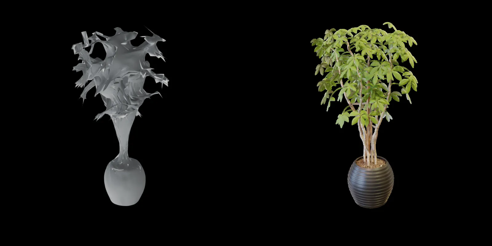
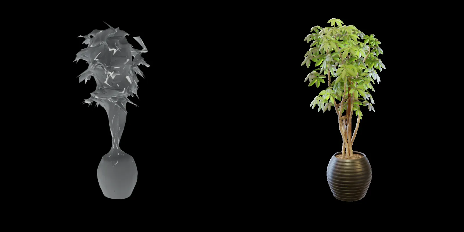
To answer these questions, I built a pipeline that deforms a sphere primitive into a target mesh using only 2D reference images. It replaces a multi-day manual modeling task with ~60 minutes of GPU compute on a GB10.
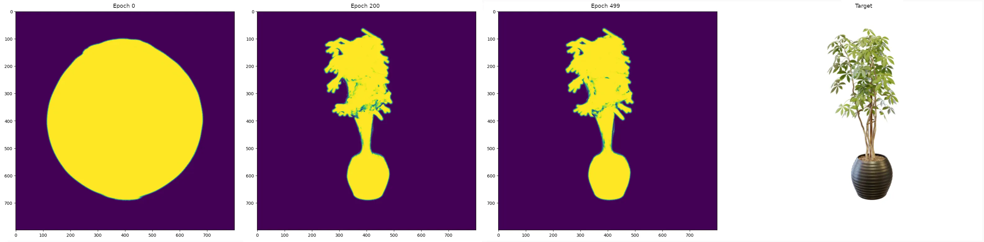 [VISUAL: Side-by-side
— initial sphere | intermediate mesh (~200 iterations) | final mesh (~500
iterations) | ground truth comparison]
[VISUAL: Side-by-side
— initial sphere | intermediate mesh (~200 iterations) | final mesh (~500
iterations) | ground truth comparison]
Workflow Overview
This is a deep dive into the mathematics, coordinate systems, and optimization strategies required to combine traditional 3D modeling with machine learning. Here’s how the pipeline works:
- Load a dataset of 2D images and their corresponding 3D camera poses (a json file with transformation matrices).
- Render a soft, differentiable silhouette of the current guess (mesh) from an exact camera pose.
- Compare the rendered silhouette to the ground-truth image mask using a custom geometric loss function.
- Backpropagate the loss through the PyTorch3D renderer and update the 3D coordinates of the mesh vertices.
- Output a final mesh in
.objformat.
This workflow is well-documented in PyTorch3D’s mesh fitting tutorial. The engineering challenge is in getting it to work for a wide range of datasets with real-world data and complex geometry.
Here are the four main design decisions that made the process converge to good results:
- Coordinate system pipeline — general-purpose conversion across Blender/NeRF/COLMAP → PyTorch3D conventions
- Soft IoU loss — replace MSE to handle class imbalance between object and background
- Dynamic loss annealing — configurable decay schedules for regularization, enabling coarse-to-fine optimization
- Multi-view batching — simultaneous gradient accumulation across camera views to prevent over-fitting
Key Design Decisions & Techniques
1. Coordinate System Pipeline
The first engineering challenge was bridging coordinate conventions. Life would be easier if everyone could agree on coordinate system conventions. Object space, camera space, world space, NDC/clip space, and screen space. All with their own orientations. Then there’s row-major (Camera-to-World) and column-major matrices (World-to-Camera). The math is straightforward. Getting the implementation correct across all the convention combinations isn’t.
The input data uses Blender/NeRF/COLMAP conventions. PyTorch3D expects row-major, left-handed NDC (Normalized-Device-Coordinate) space. These are well-understood transforms, but getting them wrong produces incorrect renders. That means it may fit to an undesired viewpoint (e.g. the bottom of the object). Even worse, the optimization may never converge (camera doesn’t point at the mesh).
Synthetic datasets are great for making sure your optimizer works, but real-world data is so much more satisfying to work with. Especially when it’s your own manual captures. From the start I knew I wanted the pipeline to handle multiple data sources. This meant that hardcoding the Blender-to-PyTorch3D transform from the NeRF/COLMAP convention wasn’t an option. Instead, I built a general conversion pipeline. It handles the full conversion chain: object → world → camera → NDC/clip → screen space. It works across both row-major and column-major conventions for common coordinate systems. This made the system reusable across datasets from different sources.
That small extra effort paid off immediately when I used my own ground-truth captures with COLMAP poses. The pipeline handled the different coordinate system without any changes.
If you’re not sure if the coordinates are correct (or are a visual thinker like me), I also built camviz, a camera matrix visualizer for debugging coordinate issues visually.
2. Why Soft IoU Over MSE?
The standard approach for silhouette comparison is MSE (Mean-Squared-Error) loss. It’s fraught with issues though (see the SSIM paper for interesting examples of perceptual quality vs MSE). When using it, the optimization was converging very slowly. After 700 iterations the mesh volume was still 2x too large.
This was due to the “class imbalance” problem. Depending on camera distance and framing, the target object can occupy a small fraction of the rendered image. MSE gets dominated by the vast “correctly empty” background. This produces weak gradients on the actual object boundary. That in turn leads to small updates and slow convergence.
I implemented a differentiable Soft IoU (Intersection-over-Union) loss instead. IoU does a good job of focusing the loss on the geometric overlap between the prediction and the target. It completely ignores “empty” pixels (true negatives).
The “soft” component matters here. PyTorch3D’s silhouette renderer is differentiable via “soft” (varying opacity) edges which allow for tiny updates to the mesh. The loss uses a small tweak to handle these soft boundaries. This stops them from dominating the gradient signal. It forces the mesh to expand and contract regardless of the object’s size on screen.
With soft IoU, it took only 50 iterations for the mesh volume to converge to the correct size. A dramatic 14x improvement compared to MSE’s 700+ iterations. This meant that the optimizer could spend more of its budget on shape refinement.
3. Dynamic Loss Annealing & Regularization
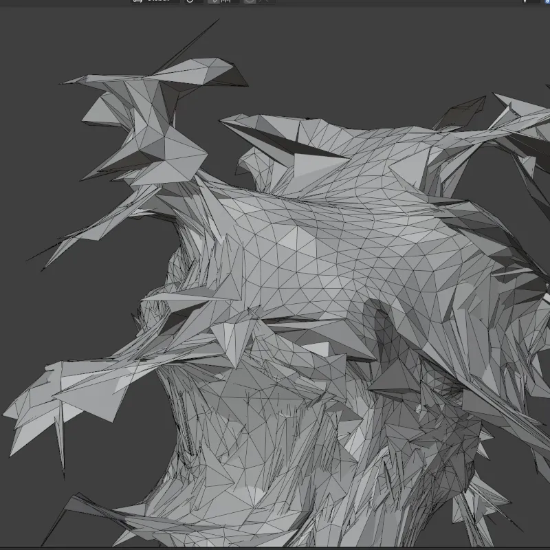
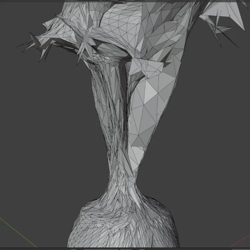
Silhouette loss alone produces broken meshes, and often crashes PyTorch3D’s differential solver. The optimizer will “explode” the mesh into jagged, self-intersecting geometry. It may project well in 2D but is unusable in practice. This happens when the vertices get pushed apart into a spiky mess to match the 2D views.
Three regularization terms prevent this:
- Laplacian Smoothing: Prevents vertices from moving too independently, keeping the surface smooth.
- Normal Consistency: Ensures neighboring faces point in similar directions.
- Edge Length Penalty: Prevents any single triangle from stretching infinitely.
Each of these regularization terms has different importance in the overall result. Therefore the losses are weighted (scaled) before summing with the silhouette loss. Getting the balance of the weights is tricky. Too much silhouette loss and the differentiable renderer would crash after 50-100 iterations. Too much regularization and 600 iterations later the mesh still doesn’t have a recognizable shape.
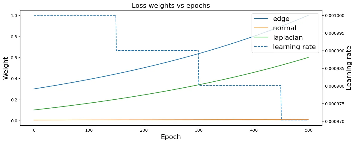
The key design decision was making the regularization weights dynamic rather than fixed. I implemented configurable annealing schedules: static, linear, cosine, and exponential decay. They can be set independently per regularization term.
The choice of schedules is a significant factor. Linear decay kept the optimization stable, but the mesh would “stall-out” (little-to-no progress). Switching to cosine and exponential decay resulted in better results. The mesh continued to progress well into the “fine detail” phase.
These faster decaying schedules enabled a clear two-phase optimization in one continuous run:
- Iterations 0–100: High silhouette weight drives large topological changes. Relaxed regularization allows for major vertex displacement. This pushes massive structural changes early on.
- Iterations 100–1000: Regularization weights increase (or silhouette weight decays). This emphasizes fine detail and mesh quality. It locks in the high-frequency details as optimization converges.
The real challenge is that with 4 different losses with 4 different decay schedules, and a learning rate with its own schedule, it takes a lot of trial and error to find the ideal combination. The annealing schedule takes a pipeline that fails on complex geometry and makes it converge to usable meshes.
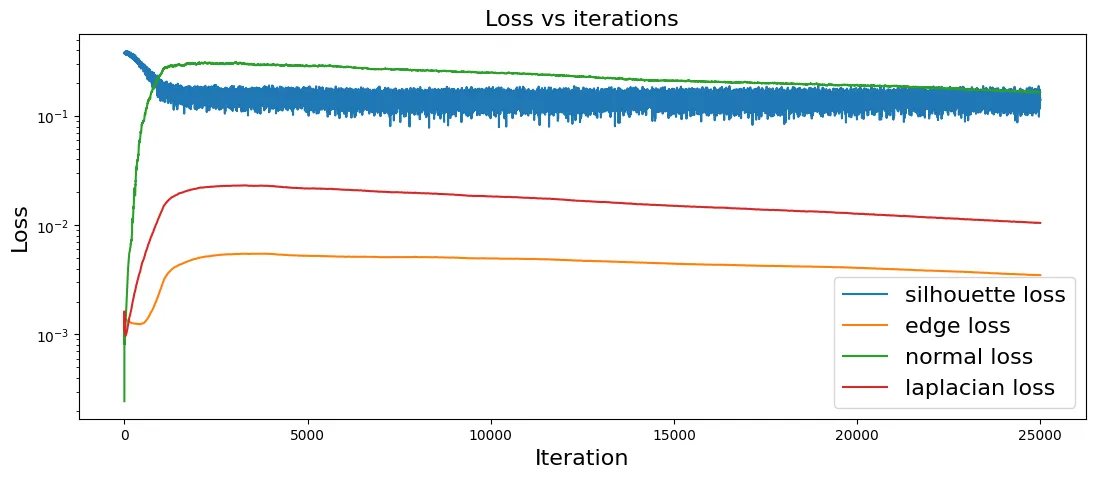
 [VISUAL:
Loss curves showing silhouette loss vs. regularization losses over 500
iterations, with annealing phases visible]
[VISUAL:
Loss curves showing silhouette loss vs. regularization losses over 500
iterations, with annealing phases visible]
4. Multi-View Batching for Stability
Single-view optimization is a trap. Fitting to one camera at a time causes the mesh to “fight itself”. Vertices get smashed to match one view, then yanked in the opposite direction for the next. This destabilizes training and the resulting mesh oscillates and converges very slowly (if at all).
The solution is to process multiple camera views simultaneously. Explicit tensor
expansion (mesh.extend()) preserves the computation graph. The gradients from
all views can then accumulate back to the single set of learnable vertex
parameters. The batch size (number of cameras) controls the strength of this
stabilization effect. Larger batches smooth the gradient signal and prevent a
single view from dominating. This is essential for convergence on geometrically
complex targets.
I began with a batch size of 4. My reasoning was that four orthographic views would provide good coverage. With random batch shuffling you’re not guaranteed to get differing views though (it’s not clear if that’s desired). After 400 iterations the starting sphere had barely changed. Dropping to 2 views per batch resulted in large changes within the first 100 iterations with no oscillation issues.
Results & Reflections
| Metric | Value |
|---|---|
| Hardware | NVIDIA GB10 GPU |
| Total runtime | ~60 min (500 iterations) |
| Per-step time | ~0.21 sec |
| Peak VRAM | 3365 MiB |
Sample Set Metrics
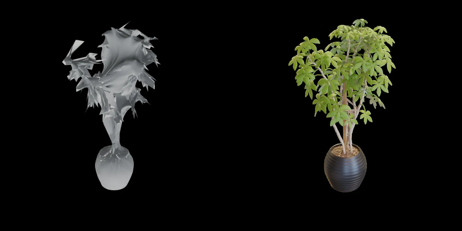
[VISUAL: Final mesh renders alongside ground-truth reference images from same angles | rendered with recon-bench]
Image Metrics
| 📊 Metric | Mean |
|---|---|
| psnr | 17.1591 |
| ssim_windowed | 0.8441 |
| lpips | 0.1714 |
Image Metrics (per item)
| 📊 Item | psnr | ssim_windowed | lpips |
|---|---|---|---|
| [0] | 16.3373 | 0.8287 | 0.1892 |
| [1] | 16.9737 | 0.8509 | 0.1708 |
| [2] | 18.1515 | 0.8694 | 0.1353 |
| [3] | 17.1741 | 0.8275 | 0.1904 |
What the Pipeline Achieved
~60 Minutes vs. Days of Manual Work
The pipeline takes a sphere, 2D reference images, and camera poses as input, and outputs a .obj mesh that preserves the major geometric features of the target. It’s the kind of output I wished I’d had during that self-portrait project — either immediately usable or a strong starting point for manual refinement. At 0.21 sec/iteration and 3365MiB VRAM on a GB10, longer optimization runs on less powerful consumer hardware are well within reach.
Two-Phase Optimization from a Single Run
The loss curves show a clear split: rapid structural convergence in the first ~100 iterations, then steady surface refinement over the remaining 400.
Recognizable Geometry, Usable Topology
The final mesh is immediately identifiable from any viewing angle. Edge uniformity, face normals, and surface smoothness are good enough for use cases where topological accuracy matters, or as a base for further refinement.
Cross-Dataset Compatibility
The system worked on both synthetic NeRF/Blender datasets and my own real-world COLMAP captures without modification.
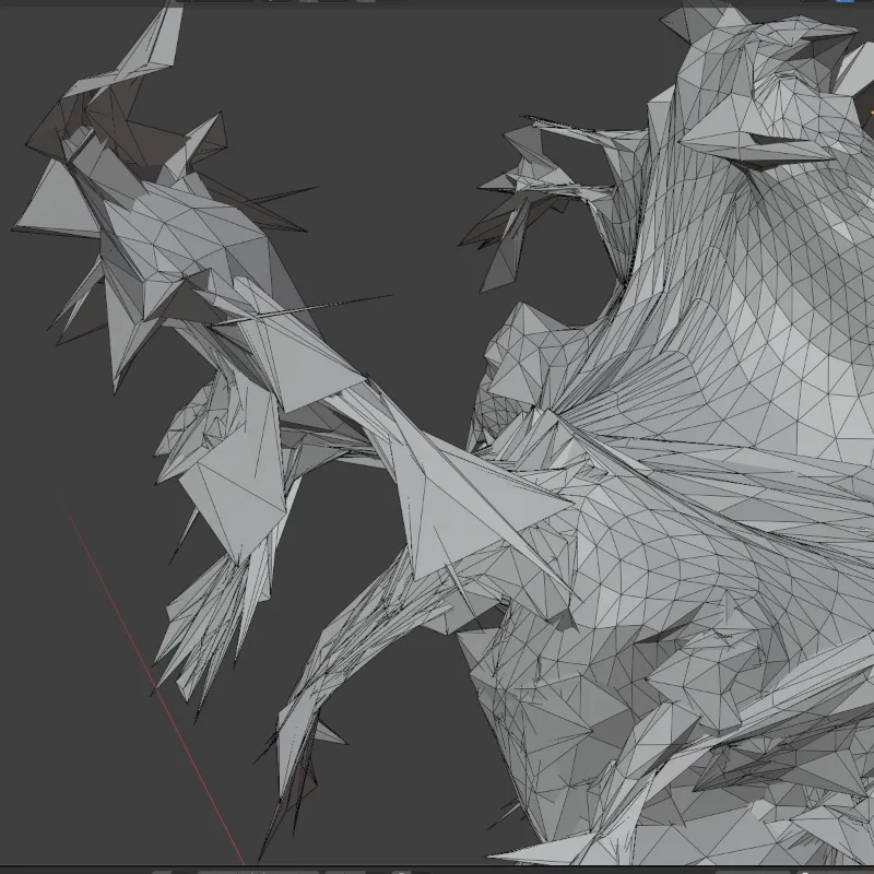
[VISUAL: Close-up comparison — areas where the mesh captures fine detail well vs. areas where it approximates]
The Brutal Truth
Given the complexity of the target, this method resulted in a good (but not great) mesh. The object is immediately recognizable in both 3D and silhouette. It would still need textures for a proper rendered appearance. As a tool for generating an approximation, or for a base mesh to be refined by hand, it’s an excellent output. As a production ready final mesh for complex shapes, it’s still lacking.
It might be a little obvious, but it bears stating. This system has no generative capabilities. If it’s not explicitly in the source images, it won’t get modeled. This means the output relies heavily on the quality of the input data. There’s no way to compensate for sparse or noisy captures.
Instant feedback is one of the most enjoyable parts about mesh fitting. As the system runs, it’s very easy to visualize the progress of the optimization. There are no held-out evals. You don’t have to decipher feature/attention maps. There’s no waiting for the full training run before seeing if something worked. You can watch the sphere deform in (almost) real time. You can see the exact render that is being used to calculate the loss. Even the failed experiments are satisfying.
The Parameter Tuning Problem
Compared to standard Machine Learning, parameter tuning for 3D can be much more challenging. I’m not talking about trying to hold 3D shapes in your head (which isn’t easy either). The hard part is the lack of numeric feedback and the massive combinatorial space.
The combinatorial space of annealing schedules × regularization weights × batch size is very large. A low loss doesn’t guarantee a good mesh either. It’s not difficult to end up with a low loss with a “bad” mesh. With a 2D image task, “low quality” results usually manifest themselves in an easy to see way. A “bad” mesh can look good visually, but cause downstream problems for texturing, deformations, and scaling. These issues are also not universal. Different use cases call for varying mesh qualities. Smooth surfaces for rendering vs. accurate topology for simulation vs. uniform faces for subdivision. Opposing objectives complicate this further. Aggressive smoothing destroys detail and shorter edges need higher face counts.
What this means in practice is a lot of trial and error plus visual inspection. This is not intuitive. What does a slowly increasing laplacian loss look like when combined with a fast moving edge loss?
I’ve been experimenting with some novel ways to explore parameter tuning beyond the usual grid/random search. The regularization weight problem is a multi-objective optimization. Smoothness, detail, and edge uniformity compete with no “best” solution. I’m exploring Pareto front configurations…More on that soon!
Fixed Mesh Resolution
The current pipeline operates on a fixed-resolution mesh. A lower resolution mesh results in faster optimization. But then it may not have enough triangles to capture the target detail. Adaptive subdivision (starting coarse and refining in regions of high silhouette error) can add detail without the computational cost of a globally dense mesh. This enables designing the mesh to capture the target’s unique shape.
3D Vision vs. Deep Learning
The lines between 3D Vision and Deep Learning are becoming more blurred as Machine Learning methods and techniques get added to the mix. However, the two domains remain fundamentally different in how you work with them.
This project sits on the 3D vision side of things. It has explicit geometry, deterministic optimization, and direct inspection at every step. 3D (vision, graphics, perception, etc) has a spatial component that feels very intuitive for visual thinkers like me. You can directly translate numbers to “real” things: add 2 to the x-dimension → shift something by 2 units. Interpretability becomes a simple visualization exercise. Not sure what’s happening to a mesh? Render a view of it. Can’t figure out if your camera is moving the desired direction? Graph it. Very often it’s a nice linear process.
Of course this does make it sound a lot cleaner than it is. This work may be happening in a 3D “space”, but you view it on a 2D screen (although I expect this to change as headsets improve). Your brain is going to have to do a significant amount of work to interpret what you see into three dimensions. This can be difficult for some people. You’ve probably seen examples of optical illusions where you can’t tell if something is pointing towards or away from you.
If you’re fortunate enough to not struggle with the visual elements, then the ability to continually inspect components at any point in the pipeline is a real gift. It’s what makes 3D vision feel very “tangible” and direct.
Working with generative diffusion models (and most of Deep Learning) feels distinctly different to this. Like with vision, final outputs can also be images that represent 3D space. But the models aren’t restricted to operating in three dimensions. The high dimensional spaces that they use feels like a “black box”. It’s because it’s impossible to visualize them (for a human). You can look at feature/attention maps, do PCA and graph the results, but they’re approximations of what’s happening.
Probability density modeling (what diffusion models do) though, feels more like a guessing game. This is because everything relies so much on statistical probabilities. You change some parameters, adjust the data distribution, and (hopefully) increase the probability of the model generating the desired result.
This doesn’t mean you’re flailing about making guesses. Good research and experiment design allows you to increase the certainty around the changes that you make. But you do have to be comfortable with uncertainty and not knowing. That’s what ultimately makes it feel like a very indirect process.
We’re starting to see the two domains converging. Production pipelines are increasingly mixing explicit geometry with learned components. Methods like SDS (Score Distillation Sampling) use diffusion priors to guide 3D optimization. Having worked in both, I find it easier to judge which approach better fits a given problem:
- Known camera poses with good coverage → 3D reconstruction and direct optimization of explicit geometry is a clear winner.
- Sparse views, novel object categories, texture generation → learned priors start to make more sense.
- Hybrid pipelines → where 3D vision seems to be heading.
3D Vision and Deep Learning are challenging in their own ways, and each is better suited to certain types of thinkers. I do enjoy thinking in concepts and abstractions as required by neural networks. However, the more “concrete” nature of 3D appeals more to my “get in there with your hands and fix it” approach to problem solving. As these two domains continue to merge, success will come from being able to switch between the two ways of thinking.